

What the Evidence Shows
- In this January 1960–June 2026 sample, equity total-return wealth grew about 815 times in nominal terms and 71.5 times after CPI. Inflation reduced the gain; it did not erase it.
- From December 1971 to December 1979, nominal total return was +51.2%, while CPI-adjusted total return was -19.0%.
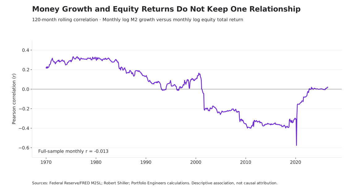
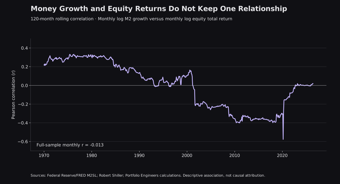
- Monthly M2 growth and equity log returns have a full-sample correlation of -0.013. Relationships across periods and rolling windows vary considerably.
- Gold-relative and M2-relative performance can challenge the dollar narrative, but neither is a consumer purchasing-power measure or a causal explanation.
The Account That Doubled
Imagine opening an investment account with $100,000. Ten years later, the statement reads $200,000. No additional contributions, no withdrawals. You have twice as many dollars. The obvious conclusion is that your wealth doubled.
Now suppose the consumer price level increased by 40% over those ten years. The ending balance buys what approximately $142,857 bought at the beginning. Your purchasing power increased by about 42.9%, rather than 100%. That is meaningful progress. It is also a different result from the one the account statement appears to describe.
Starting Balance
$100,000
Ending Nominal Balance
$200,000
Ending Purchasing Power
$142,857
This is a hypothetical example, not a historical backtest. Its arithmetic is simple: divide the ending balance by 1.40. The difficult part is deciding which question matters. Do you want to know how many dollars you have, how much consumption they support, how the investment performed against another asset, or what the underlying businesses earned?
Those questions overlap without being interchangeable. A stock portfolio can create genuine economic value while benefiting from inflation and investors paying higher valuations. It can beat consumer prices while losing ground to gold. It can rise faster than the money supply without proving that monetary conditions were irrelevant.
The illusion begins when one measurement is asked to answer every question. Our purpose is to separate those measurements, examine the history, and connect the result to the actual job an investment is supposed to perform.
The Measuring Stick Problem
Nominal returns dominate investing for a practical reason: financial obligations are usually settled in currency. Companies report dollar earnings, investors receive dollar distributions, and account statements show dollar balances. A $200,000 balance can pay a $200,000 bill. Nominal measurement is necessary.
But a dollar is not a fixed quantity of consumption. When the price level rises, more dollars are required to purchase the same broad basket of goods and services. The exact real-return relationship is (1 + nominal return) ÷ (1 + inflation) − 1. Subtracting inflation from a nominal return is a useful approximation for small changes; it becomes less accurate over long periods or large moves.
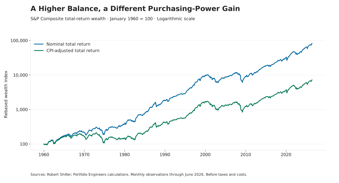
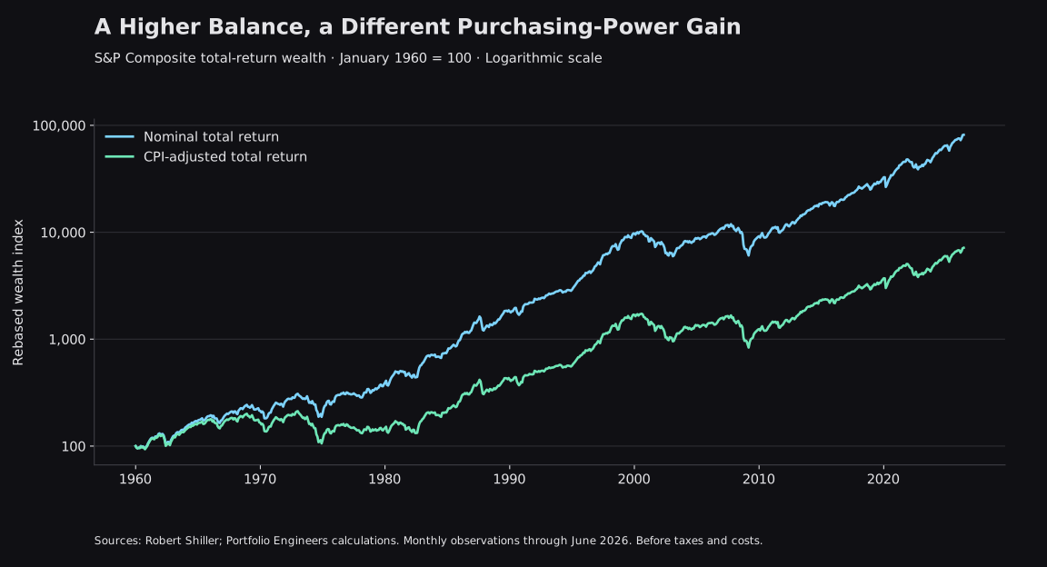
Across the full aligned sample, nominal total return annualized at 10.62%, compared with 6.64% after CPI. The difference compounds for more than six decades. It is substantial enough to change how the outcome should be described, but the real gain remains substantial too.
The path matters as much as the endpoint. In this monthly CPI-adjusted total-return history, the January 1973 peak was not recovered until January 1985. The August 2000 peak was not recovered until May 2013. These were 144- and 153-month waits, measured from a prior monthly peak to the first monthly observation at or above it. Reinvested dividends helped, but did not eliminate the experience of spending years below an earlier purchasing-power high.
These are historical descriptions of one U.S. equity series. Monthly averages smooth daily extremes, and a different starting month, inflation measure, or distribution convention can change the dates. Nor does recovery of an index mean an investor spending from the portfolio recovered on the same schedule. Withdrawals, taxes, and behavior can alter the personal outcome.
This is why the distinction is useful for planning. A future obligation denominated in a changing cost of living requires more than a nominal growth target. At the same time, a real-return chart should not be mistaken for a guarantee that equities will protect purchasing power over every investment horizon.
Four Views of the Same Investment
We use one equity history below and change its reference measure. The investment is the S&P Composite series published by Robert Shiller, using his supplied total-return history and associated CPI. Gold comes from the World Bank’s monthly commodity series; M2 comes from the Federal Reserve through FRED. These are separate source histories aligned by observation month.[1][2][3]
Change the Measuring Stick
Same equity history, different references. Every view starts at 100; changing the unit changes the question.
Equity wealth divided by the change in CPI. This estimates purchasing power against a broad consumer basket, not your personal spending pattern.
Jan 1960 – Jun 2026 · Total Return · Log Scale · Starting Value 100
Solid: Consumer Purchasing Power · Dashed: Nominal Equity Wealth · Hover, Tap, or Use Arrow Keys to Inspect
- Cumulative Change in This View
- +7,054.90%
- Annualized Change in This View
- +6.64%
- Largest Decline in This View
- -51.76%
Sources: Shiller, World Bank, Federal Reserve/FRED; Portfolio Engineers calculations. Monthly averages and interpolated fundamentals; before taxes and costs. Gold changes reference methodology in June 2025. Gold- and M2-relative changes are ratio changes, not consumer purchasing-power returns. See methods below.
The dollar view answers the account-value question. It measures the equity investment’s nominal wealth growth. With dividends included, the investment is a reinvested total-return index. With the checkbox cleared, it becomes price-only performance. That distinction should come before any comparison with inflation, gold, or money growth.
The CPI view asks how equity wealth changed relative to a broad consumer basket. It is the closest of these four views to a general purchasing-power measure. It still does not describe every household’s costs. A retiree paying substantial medical bills and a household with a fixed-rate mortgage may face different spending pressures even when they see the same headline inflation rate.[4]
The gold view asks how much gold the equity wealth could purchase relative to the starting month. A declining line can mean equities fell, gold rose faster, or both. Gold has no corporate earnings stream and its own price reflects changing demand, expectations, and supply conditions. Its usefulness as a reference does not turn it into a stable consumption basket.
From December 2022 through June 2026, for example, the equity total-return index gained 99.7% in dollars and 77.5% after CPI, yet its gold-relative value changed by -15.1%. All three statements can be true. The first describes dollar wealth; the second describes broad consumer purchasing power; the third describes an opportunity cost against another asset.
The M2 view divides equity wealth growth by growth in a monetary aggregate. M2 is a stock of money and liquid deposits, measured here in billions of dollars and seasonally adjusted. It is not a basket of prices, the Federal Reserve’s balance sheet, total credit, or the market value of all assets. A normalized equity-to-M2 ratio is therefore an exploratory relative measure.[3][6]
Over the full sample, equity total-return wealth grew 10.5 times relative to M2. That does not mean an investor owned a larger share of the money supply: an index return and an economy-wide money stock are not matching claims on the same pool. It also does not identify which part of the equity gain was caused by monetary expansion.
The choice of reference can change the visual story dramatically. The analytical discipline is to keep the label attached to the result. Consumer purchasing power, relative asset performance, and monetary-relative performance deserve different names because they answer different questions.
Money Growth and Market Returns
Overlay a long equity index with a long M2 series and the monetary explanation can appear self-evident. Both lines trend upward. Both grew dramatically around some major economic transitions. But two rising levels are a weak basis for deciding why returns occurred. Population, nominal output, earnings, and many other economic quantities also grow over time.
A more informative first check compares changes. We calculated monthly log equity total returns and monthly log M2 growth on matching observation months. Across 797 monthly pairs from February 1960 through June 2026, their contemporaneous Pearson correlation is -0.013. In this simple specification, knowing whether monthly M2 growth was larger provides very little linear information about that month’s equity return.
That result does not establish that monetary policy has no effect. M2 growth is not the same variable as an unexpected interest-rate decision, a change in credit availability, or a shift in investors’ expectations. A market can respond to anticipated policy before a monetary aggregate is published. Policy can also respond to worsening conditions that are already damaging asset prices.
There are plausible mechanisms behind a monetary influence. Lower financing costs can support investment and demand. Changes in the rates used to discount future cash flows can alter valuations. Investors may reallocate among deposits, bonds, and equities as relative yields and risks change. Expectations about inflation, profits, and future policy can move at the same time.[5]
A simple valuation example illustrates one channel without proving its historical magnitude. A hypothetical perpetual $10 annual cash flow is worth $200 at a 5% discount rate and about $167 at 6%, assuming the same cash flow and risk treatment. A lower price need not mean the asset suddenly produces less; it can mean investors require a higher return. Real businesses have uncertain, changing cash flows, so this is an illustration rather than an equity-pricing model.
Causal monetary-policy research uses identification methods designed to separate policy surprises from other news and from the central bank’s response to the economy. Rigobon and Sack’s Federal Reserve staff paper makes precisely that distinction. Our monthly correlations do not replicate that exercise and cannot assign an exact share of market appreciation to monetary policy.[7]
| Observation Months | Nominal Total Return / Year | CPI-Adjusted / Year | Monthly M2 / Equity r |
|---|---|---|---|
| 1971-12 – 1979-12 | 5.30% | -2.60% | 0.279 |
| 1981-12 – 1999-12 | 18.19% | 14.43% | 0.075 |
| 1999-12 – 2009-12 | -0.73% | -3.17% | -0.357 |
| 2008-12 – 2019-12 | 14.74% | 12.66% | -0.328 |
| 2019-12 – 2022-12 | 8.92% | 3.81% | 0.055 |
| 2022-12 – 2026-06 | 21.85% | 17.82% | 0.189 |
The selected episodes deliberately include conflicting outcomes. During December 1971–December 1979, money growth accompanied a positive nominal equity return but a negative real return. During December 1999–December 2009, M2 increased while equity total-return wealth declined. In the recovery beginning at December 2008, strong equity gains coexisted with a negative contemporaneous monthly correlation.
The pandemic interval is another reminder about endpoints. December 2019–December 2022 combines an extraordinary expansion, a reopening, an inflation shock, and tightening into one measurement. It cannot tell us whether the same mechanism dominated every stage. The recent interval also differs from the full history; it is too short to establish a new permanent relationship.
We checked several offsets as a sensitivity exercise. Correlations between this month’s M2 growth and equity returns one, three, or twelve months later are approximately 0.06, 0.05, and -0.04. Those results are small in this specification. They are not forecasts: the analysis uses revised observation-month data, not the releases that an investor actually had in hand.
The practical conclusion is narrower than either popular narrative. Monetary conditions can matter without making a money-stock chart a complete explanation of equity prices. A weak full-sample correlation does not dismiss the transmission mechanism; a strong correlation in one episode would not prove a universal one.
What Actually Drove the Return?
Stocks are ownership claims on businesses. A business can sell more units, develop a useful product, improve its margins, expand internationally, or use capital more effectively. Owners can receive cash along the way. These are reasons an investment can become more valuable beyond a change in the currency used to quote it.
Yet the quoted price is also what another investor is willing to pay for that claim. Earnings can grow while a stock price stagnates if the valuation multiple falls. A stock price can rise faster than earnings if investors become willing to pay more for each dollar of profits. These effects can reinforce one another or cancel out.
For positive endpoint earnings, the accounting identity is exact: price = earnings per share × price/earnings multiple. In log terms, price growth is the sum of earnings growth and the change in the P/E multiple. Add the log difference between total-return wealth growth and price growth, and the result reconciles to total return.
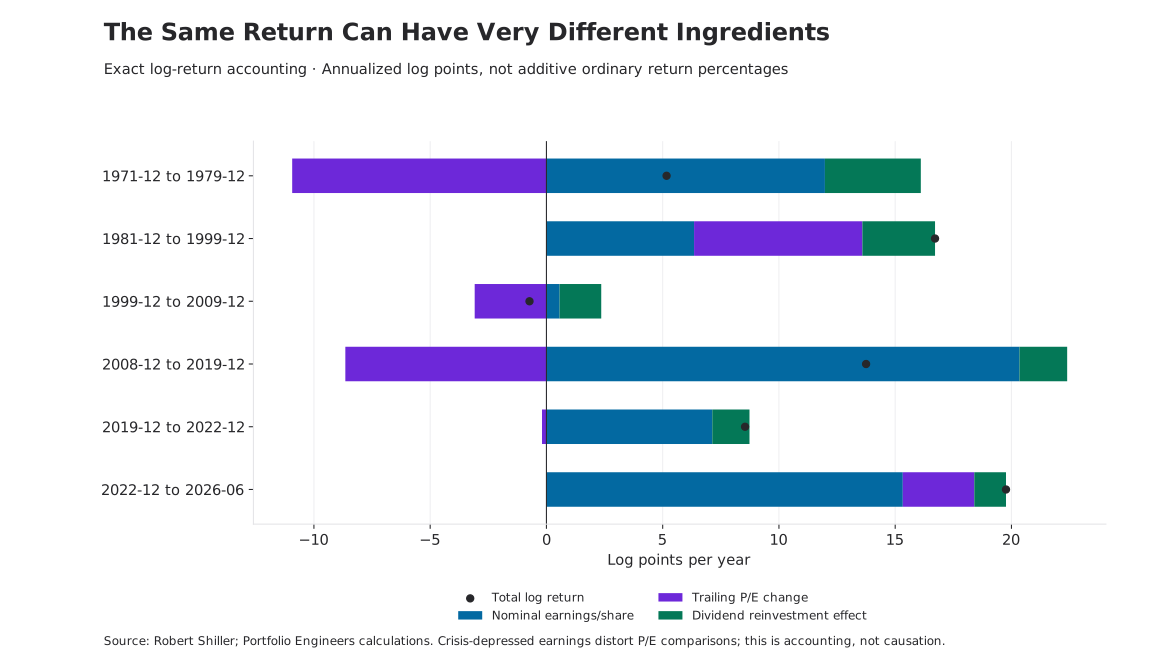
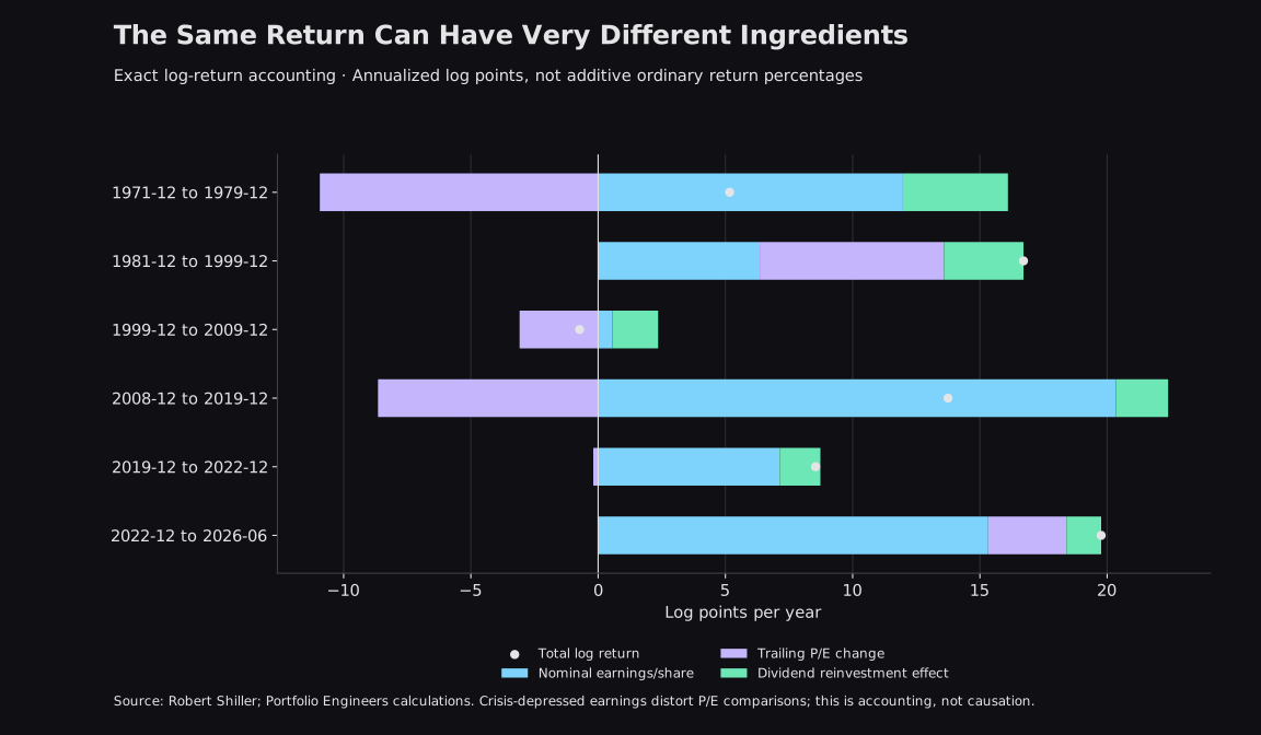
From December 1981 through December 1999, equity total return annualized at 18.19%. Both nominal earnings growth and multiple expansion contributed materially in this accounting. Calling the entire rise productive growth would overlook the valuation component. Calling it entirely monetary illusion would overlook earnings and distributions.
The next decade looks different. From December 1999 through December 2009, price return was -22.3%, while reinvested total return was -7.0%. Trailing earnings ended only modestly above their starting level and the P/E multiple compressed. Dividends softened the loss. They did not make the experience equivalent to a healthy compounding decade, especially after inflation.
The recovery comparison contains a trap worth making visible. December 2008 is a crisis-depressed earnings base. From that starting point, the accounting attributes very large growth to earnings and a negative contribution to the P/E change, even while the market rises strongly. That does not establish that investors became more pessimistic. A trailing P/E can fall simply because depressed reported profits recover faster than prices.
Nor is nominal earnings growth the same as productivity growth. Inflation can raise reported revenue and profits. Share repurchases can increase earnings per share without an equivalent increase in aggregate business output. Index membership changes over time. This decomposition tells us how the return reconciles, not how much society became richer through innovation.
The broader dividend point is visible in the full history too. Price-only appreciation annualized at 7.58%, versus 10.62% for total return. That difference is why an equity-versus-inflation comparison should specify whether shareholders reinvested their distributions. A price index and a reinvested wealth index describe different experiences.
Asset Prices and Consumer Prices
Consumer inflation and rising asset prices are often placed under the same heading, but the measurements differ. CPI tracks consumer goods and services. Stocks and bonds are investment items, not direct components of that consumption basket. For owner-occupied housing, the CPI shelter measure uses rental equivalence rather than treating the purchase price of a house as current consumption.[4][8]
This leaves room for a period of relatively modest consumer inflation alongside substantial asset appreciation. Expected earnings, financing conditions, risk premiums, and the price investors attach to future cash flows can change without an equivalent change in today’s grocery or electricity bill. Conversely, higher living costs can coincide with declining asset valuations.
Calling the first experience “asset inflation” can be a useful description of rising market prices. It does not by itself identify monetary debasement as the cause. A company earning sustainably higher profits and a company trading at a temporarily elevated multiple can both produce a rising stock chart, despite very different underlying conditions.
Ownership changes the household experience as well. Two households can face similar increases in living costs while experiencing different changes in their balance sheets. One may hold mostly cash; another may own equities or property. Asset appreciation benefits the owners of those assets, while making acquisition more expensive for a prospective buyer.
That observation needs context. The households may also differ in savings rates, debt, income, taxes, spending needs, and the risks they accepted. Leverage can amplify gains and losses. A rising house price does not automatically give an owner more cash to spend, and selling an appreciated asset may bring tax or replacement costs.
For an investor, CPI is therefore an essential reference rather than a complete personal financial plan. A broad inflation adjustment can show whether a portfolio gained purchasing power in general. It cannot alone tell a first-time homebuyer how close they are to a deposit, or a retiree whether their particular expenses remain covered.
What Should Success Mean?
An investment exists to support something beyond its own quoted price. That may be retirement spending, a near-term purchase, financial flexibility, or the capacity to absorb an unexpected expense. The appropriate measurement follows that purpose.
Nominal growth asks whether the dollar balance increased. Real growth asks whether it buys more against a stated spending reference. Relative performance asks whether the strategy beat an appropriate alternative. Risk asks what drawdowns, uncertainty, and liquidity constraints accompanied the outcome. Goal achievement asks whether the money can meet the obligation it was intended to fund.
It is possible to succeed on one dimension and fail on another. A portfolio can beat inflation while lagging a suitable market benchmark. It can beat that benchmark while exposing its owner to a drawdown they cannot tolerate. It can recover eventually while failing someone who needed to withdraw during the decline.
This is where the research connects to Portfolio Engineers’ design philosophy. Distinct financial roles should not be forced into one contest for the highest historical return. Our portfolio mandates describe different jobs, not three conclusions proven by the charts in this article.
Adaptive Regime Core (ARC) is a diversified, equity-centered foundation for long-term compounding, with complementary exposures intended to behave differently across environments. The relevant questions include real growth over time, concentration, resilience, and whether the allocation remains consistent with its rules.
Higher-Yield Savings (HYS) serves a liquidity and income role. Its evaluation should emphasize flexibility, the behavior of the underlying holdings, and the investment horizon. The word “savings” does not make a market portfolio equivalent to an insured bank deposit or guarantee purchasing-power preservation.
Asymmetric Growth (AG) pursues higher-risk growth opportunities with the possibility of disproportionate upside and substantial losses. That role calls for explicit risk limits and expectations about volatility. A strong nominal period does not establish that the allocation is appropriate for near-term spending.
The Regime Dashboard offers a related way to organize current inflation, liquidity, risk preference, and growth conditions. It is a framework for interpreting the environment, not a mechanism for separating every market return into its true economic causes. Our early regime-return study makes the same distinction between an interesting historical association and validated predictive information.
Return to the investor whose account reached $200,000. The higher balance matters. So does the purchasing power it represents, the risks taken to reach it, and the obligations it can now support. Neither dismissing the gain as an illusion nor accepting the nominal number as the whole story is a sufficient assessment.
Markets are priced in dollars. Investment success is experienced through consumption, ownership, resilience, and the ability to meet future commitments. The useful question is not which measuring stick is perfect. It is what each measurement reveals, what it leaves out, and whether the investment is doing the job it was designed to do.
Methods, Downloads, and Sources
Capture and coverage. This is a frozen October 20, 2026 research capture with 798 consecutive monthly observations from January 1960 through June 2026. June is the latest shared month with complete price, CPI, earnings, dividend, gold, and M2 inputs under our completeness rule. More recent prices or estimated consumer-price observations in a source workbook do not extend this sample.
Equity and inflation series. We use Shiller’s monthly S&P Composite price, nominal trailing dividends and earnings, CPI, and supplied real total-return wealth index. Nominal total-return wealth is recovered by multiplying that real wealth index by CPI, then rebasing. Price-only and total-return comparisons are kept separate. Prices are monthly averages, not month-end closes; earnings and dividend figures include interpolation from quarterly totals. The index is not one continuously held fund, and the study does not include fund expenses, investor taxes, transaction costs, withdrawals, or additional contributions.[1]
Gold and money. World Bank gold prices are monthly U.S.-dollar averages per troy ounce. The workbook changes from London afternoon fixing averages to spot-price averages in June 2025; the series is not one unchanged benchmark throughout. Early gold observations also span a different monetary and convertibility setting. M2SL is seasonally adjusted and uses the captured revised history. Federal Reserve definitions and revisions matter; M2 is not treated as the monetary base or as a consumer-price deflator.[2][3][6]
Alignment and calculations. The preparation script rejects missing shared months rather than interpolating or carrying them. Each view is rebased to 100 at the same starting month. Annualization uses the exact number of month intervals divided by twelve. The worst decline is measured within the selected rebased monthly path; in gold or M2 mode it is a decline in that ratio, not a dollar portfolio drawdown. Historical underwater episodes use the CPI-adjusted total-return index.
Statistical limits. Correlations use monthly log changes, not trending index levels. Rolling estimates use 120 observations. Positive offsets compare M2 growth with a later monthly equity return; negative offsets reverse that timing relationship. Boundaries change the sample size. These are descriptive sensitivity checks with no causal controls, no significance claims, and no out-of-sample trading validation. Revised data and observation months do not establish release-time availability.
Return accounting. With positive endpoint earnings, log total-return growth equals log earnings-per-share growth plus log P/E change plus the log total-return/price-growth difference. Dividing by years gives additive annualized log contributions. Applying the exponential to their sum converts back to an ordinary annualized return. Crisis earnings, buybacks, index changes, inflation, and interpolation all limit economic interpretations of those accounting components.
Publication scope. The interactive exhibit uses embedded frozen observations and makes no new provider requests when a reader changes its settings. The website’s shorter live histories and seasonally adjusted Backend inflation streams are not spliced into this historical study.
| Equity Return Offset | Monthly Pairs | Pearson r |
|---|---|---|
| -12 Months | 785 | 0.004 |
| -3 Months | 794 | 0.007 |
| -1 Months | 796 | -0.011 |
| 0 Months | 797 | -0.013 |
| +1 Months | 796 | 0.061 |
| +3 Months | 794 | 0.048 |
| +12 Months | 785 | -0.041 |
Sources and Reproduction
- [1] Robert Shiller · Stock Market Data
Monthly S&P Composite price, trailing earnings/dividends, CPI, and the supplied real total-return index.
- [2] World Bank · Commodity Markets / Pink Sheet
Monthly gold prices in U.S. dollars per troy ounce, including the workbook’s reference-method change.
- [3] Federal Reserve / FRED · M2SL
Seasonally adjusted monthly M2; the captured historical vintage is subject to revision.
- [4] BLS · Consumer Price Index Questions and Answers
Consumer-basket coverage, investment exclusions, and differences from an individual household’s experience.
- [5] Federal Reserve · How Monetary Policy Works
Interest rates, expectations, asset prices, and the transmission of monetary policy.
- [6] Federal Reserve · H.6 Technical Questions
Monetary-aggregate definitions and methodological changes.
- [7] Rigobon and Sack · The Impact of Monetary Policy on Asset Prices
Federal Reserve staff research on identification; its authors distinguish policy shocks from endogenous policy responses.
- [8] BLS · Rent and Rental Equivalence
How the CPI measures the consumption of shelter services rather than the investment purchase price of a home.
Portfolio Engineers owns the analysis and presentation, not the underlying providers’ data. Source workbooks and CSV captures are identified by SHA-256 in the findings download. Reproduction tooling is maintained in scripts/research/wealth-measures. Public-source histories can be revised; this publication does not update silently with the dashboards.